Leonard Chukwuemeka Anyika, Chidi Obi
ABSTRACT. This study assessed the air pollution loads of sulphur dioxide (SO2), nitrogen dioxide (NO2) and particulate matter (PM10) from Aguleri in Anambra State of Nigeria using matrix algebra and the geographical information system (GIS)/global positioning system (GPS) attachment to MATLAB. The pollutant values of SO2 and NO2 were obtained using the Crowcon Gas Monitor Model CE 89/336/EEC, while the PM10 values were obtained with the Crowcon Particulate Monitor Model No.1000 with the serial number 298621. The pollution characteristics of the study area were simulated using the polynomial expression yi = k + k1x1 + k2x2 + k3x3 +… knxn.. The predictive parameter constants, k, were determined with the solution to the simultaneous equations arising from the polynomial expressions using matrix algebra. MATLAB 7.9 curve fitting software was used to produce associated model equations from the fitted curves for the variations of SO2, NO2 and PM10 as a function of locations in Aguleri for both rainy and dry seasons. The evaluation of pollution models used for the study showed that constants from the fitted curves do not closely match constants from ab initio calculations. The corresponding coordinates in both GIS/GPS contour and surface plots revealed a pollution distribution concentration of 50% in Aguleri. The results revealed that the stations in Aguleri had a satisfactory air pollution index rating. This study serves as an improvement to air quality studies and a veritable tool for air quality management and policymaking.
Keywords: air pollutants; particulate matter; polynomial equations; seasons; software.
Cite
ALSE and ACS Style
Anyika, L.C.; Obi, C. Predictive Air Pollution Assessment Using Matrix Algebra and GIS/GPS in Aguleri Anambra State. Journal of Applied Life Sciences and Environment 2024, 57 (3), 437-458.
https://doi.org/10.46909/alse-573146
AMA Style
Anyika LC, Obi C. Predictive Air Pollution Assessment Using Matrix Algebra and GIS/GPS in Aguleri Anambra State. Journal of Applied Life Sciences and Environment. 2024; 57 (3): 437-458.
https://doi.org/10.46909/alse-573146
Chicago/Turabian Style
Anyika, Leonard Chukwuemeka, and Chidi Obi. 2024. “Predictive Air Pollution Assessment Using Matrix Algebra and GIS/GPS in Aguleri Anambra State” Journal of Applied Life Sciences and Environment 57, no. 3: 437-458.
https://doi.org/10.46909/alse-573146
View full article (HTML)
Predictive Air Pollution Assessment Using Matrix Algebra And GIS/GPS in Aguleri Anambra State
Leonard Chukwuemeka ANYIKA1 and Chidi OBI2*
1Department of Industrial Chemistry, Madonna University Elele Campus, Rivers State Nigeria
2Department of Pure and Industrial Chemistry, University of Port Harcourt, Rivers State Nigeria
*Correspondence: chidi.obi@uniport.edu.ng
Received: Jun. 02, 2024. Revised: Jul. 22, 2024. Accepted: Jul. 31, 2024. Published online: Nov. 18, 2024
ABSTRACT. This study assessed the air pollution loads of sulphur dioxide (SO2), nitrogen dioxide (NO2) and particulate matter (PM10) from Aguleri in Anambra State of Nigeria using matrix algebra and the geographical information system (GIS)/global positioning system (GPS) attachment to MATLAB. The pollutant values of SO2 and NO2 were obtained using the Crowcon Gas Monitor Model CE 89/336/EEC, while the PM10 values were obtained with the Crowcon Particulate Monitor Model No.1000 with the serial number 298621. The pollution characteristics of the study area were simulated using the polynomial expression yi = k + k1x1 + k2x2 + k3x3 +… knxn.. The predictive parameter constants, k, were determined with the solution to the simultaneous equations arising from the polynomial expressions using matrix algebra. MATLAB 7.9 curve fitting software was used to produce associated model equations from the fitted curves for the variations of SO2, NO2 and PM10 as a function of locations in Aguleri for both rainy and dry seasons. The evaluation of pollution models used for the study showed that constants from the fitted curves do not closely match constants from ab initio calculations. The corresponding coordinates in both GIS/GPS contour and surface plots revealed a pollution distribution concentration of 50% in Aguleri. The results revealed that the stations in Aguleri had a satisfactory air pollution index rating. This study serves as an improvement to air quality studies and a veritable tool for air quality management and policymaking.
Keywords: air pollutants; particulate matter; polynomial equations; seasons; software.
INTRODUCTION
Air pollution is a global phenomenon that has gradually distorted the Earth’s climate, leading to the greenhouse effect, acid rain, flooding, high temperatures, death of aquatic species, and disease spread (Abdul-Lateef et al., 2021; Abulude et al., 2024; Chengyue et al., 2021; Ilmas et al., 2018; Omokpariola et al., 2024; Tella and Balogun, 2022). Abdul-Lateef et al. (2021) reported that according to the World Health Organization (WHO), ambient and indoor air pollution have significantly increased mortality and morbidity rates, especially in developing countries. The WHO (2022) reported that the combined effects of ambient and household air pollution are associated with 6.7 million premature deaths annually, with an estimated 4.2 million premature deaths recorded worldwide in 2019, 89% of which occurred in low- and middle-income countries, particularly in the WHO South-East Asia and Western Pacific Regions.
The current population pressure in Nigeria, alongside urbanisation, modern agricultural practices, and industrialisation, has rapidly metamorphosed into air pollution (Abulude et al., 2024; Omokpariola et al., 2024). Abdulraheem et al. (2023) observed an increasing pattern in pollutants such as carbon monoxide (CO), oxides of nitrogen (NOx), particulate matter of 2.5 micrometres in diameter (PM2.5), particulate matter of 2.5 micrometres in diameter (PM10), sulphur dioxide (SO2), ammonia (NH3) and non-methane volatile organic compounds arising from the population surge in Nigeria from 1980 to 2020. The total emissions such as CO, NOx, PM2.5, PM10, SO2, NH3 and NMVOC recorded increased from 1736 to 6210 Gg, 143 to 338 Gg, 126 to 551 Gg, 171 to 717 Gg, 19 to 60 Gg, 4 to 28 Gg and 471 to 1587 Gg, respectively. The author reported that emissions from wood fuel, transportation, and municipal waste are the major sources contributing to 63%, 16%, and 15% of the total CO emissions (Abdulraheem et al., 2023). Environmental pollution modelling is a numerical tool used to describe the causal relationships between emission, discharge, and fluxes of various kinds through the natural environmental matrix. Such tools are of considerable importance in the agricultural field due to the overwhelming influence of land and water use for sustainable development (Lokeshwari et al., 2014).
The agricultural non-point source (AGNPS) pollution model was developed to analyse non-point source pollution in agricultural watersheds. Within this framework, run-off characteristics and transport processes of sediments and nutrients can be simulated for each geographical map cell routed. This permits the run-off, sedimentation, encrustations and erosion in each cell in the watershed to be determined or simulated (Luo et al., 2023; Zhu et al., 2020). Thus, AGNPS can identify sources contributing to a potential pollution challenge and prioritise those locations where remedial measures could be initiated to improve land use quality. Such modelling can be applied to air pollution studies by the incorporation of a geographic information system (GIS), global positioning service (GPS), and remote or proximate sensing (Borah et al., 2024; Firouraghi et al., 2022; Khaslan et al., 2024; Thakur et al., 2017; Utbah et al., 2023). Data from these systems can be processed in multiple dimensions on a digitised geographical map (Balogun et al., 2011; Chaminé et al., 2021; Najibullah, 2020).
In this process, GIS data layers required by models similar to AGNPS models can be created using appropriate statistical map treatment. The data generated will subsequently become spatial information for pollution studies (Khan and Jehangir, 2023; Matejicek, 2005; Tella and Balogun, 2022; Verma et al., 2023). When air pollution attributes such as NO2, SO2, PM, and ozone (O3) are available, GIS, GPS and digitised map formats can be extracted and combined with other data such as meteorological indices reformatted as needed for various geographical and best management practices in the total environment (Badach et al., 2020; Seham et al., 2022; Yerramilli et al., 2011; Yoo, 2022).
With the increase in urbanisation, industrialisation, the number of vehicles, and other anthropogenic activities, researchers have employed more sophisticated methodologies such as machine learning, artificial intelligence, and the Internet of Things to solve air pollution problems (Abdul-Lateef et al., 2021; Patra et al., 2016; Zezhi et al., 2024). Several studies of atmospheric pollution by attributes such as CO, NOx, SOx, hydrocarbons (CnH2n+2), and PM, which may or may not encapsulate metal species or volatile organic residues, have been carried out all over the world (Abdulraheem et al., 2023; Daful et al., 2020; Gerard, 2021; Jyethi et al., 2016; Knepnick and Sebastian, 1990; Manisalidis et al., 2020). Such studies, including research on emerging pollutants, are becoming widespread in Nigeria (Abam and Unachukwu, 2009; Augustine, 2012; Dimari et al., 2008; Ediagbonya and Tobin, 2013; Egbuna et al., 2021; Obisesan and Weli, 2019; Omofonmwan and Osa-Edoh, 2008; Mahmud et al., 2023; Tawari and Abowei, 2012; Yalwaji et al., 2022). However, only a handful of these studies have been able to relate physical, geographical, and meteorological data into a model which can respond to best management practices (Anyika et al., 2018). The data available so far have been only a little better than baseline statistics comparing available physical concentrations of attributes with either WHO standards or FEPA equivalents. The level of air pollution monitoring or control in Nigeria is not comparable to that of large cities like Cairo, Tehran, and Johannesburg. These countries have established regular air pollution monitoring stations for many years. Therefore, the focal point of this work is to attempt an improved interpretation of air pollution assessment using GIS, GPS, and matrix algebra.
MATERIALS AND METHODS
Description of Study Area
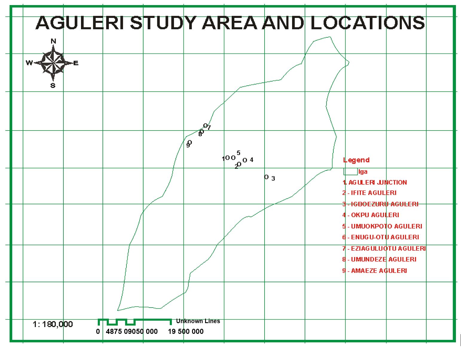
Aguleri is an area north-north-east of Onitsha town bound by the coordinates 6º20ʹ30E to E6º53ʹ, and it is 24 km NNE from Onitsha main town. Aguleri, located in the River Anambra Basin, is an agrarian town with a population of about 300,000, as represented in Figure 1. The map was obtained from Google Earth using Arc View 3.0 software. Georeferencing of all data points in maps was done using GARMIN GPS 78 s chart plotting receivers. Nine locations were designated as sampling stations in Aguleri, and each designated sampling station was divided into four sampling points from where four samples were collected. The climate of Aguleri is tropical or savanna, with two distinct dry and wet seasons. It has an annual temperature of 87.66º, 1.46% higher than Nigeria’s average temperature, with annual precipitation of 8.92 inches and 71.12% of rain annually. Aguleri has an elevation of zero feet above sea level. The points in each station have been georeferenced to enable the application of GIS/GPS analysis parameters summarised in Table 1 and Table 2.
Table 1
Georeferenced Coordinates for the Rainy Season in Aguleri
|
Sampling Station |
Coordinates |
|||
|
Point 1 |
Point 2 |
Point 3 |
POINT 4 |
|
|
Aguleri Junction |
N06º19.757ʹ E006º52.628ʹ |
N06º19.755ʹ E006º52.601ʹ |
N06º19.693ʹ E006º52.612ʹ |
N06º19.689ʹ E006º52.640ʹ |
|
Ifite Aguleri |
N06º19.354ʹ E006º53.212ʹ |
N06º19.371ʹ E006º53.188ʹ |
N06º19.376ʹ E006º53.212ʹ |
N06º19.356ʹ E006º53.194ʹ |
|
Igboezuru Aguleri |
N06º18.666ʹ E006º54.622ʹ |
N06º18.666ʹ E006º54.650ʹ |
N06º18.650ʹ E006º54.645ʹ |
N06º18.677ʹ E006º54.631ʹ |
|
Okpu Aguleri |
N06º19.584ʹ E006º53.514ʹ |
N06º19.563ʹ E006º53.547ʹ |
N06º19.599ʹ E006º53.538ʹ |
N06º19.562ʹ E006º53.524ʹ |
|
Umuokpoto Aguleri |
N06º19.758ʹ E006º52.933ʹ |
N06º19.738ʹ E006º52.966ʹ |
N06º19.736ʹ E006º52.949ʹ |
N06º19.773ʹ E006º52.963ʹ |
|
Enugu Otu Aguleri |
N06º32.134ʹ E006º55.279ʹ |
N06º32.087ʹ E006º55.300ʹ |
N06º32.029ʹ E006º55.319ʹ |
N06º31.366ʹ E006º55.344ʹ |
|
Ezi Agulu Otu Aguleri |
N06º21.480ʹ E006º51.499ʹ |
N06º21.489ʹ E006º51.517ʹ |
N06º21.496ʹ E006º51.492ʹ |
N06º21.450ʹ E006º51.496ʹ |
|
Umundeze Aguleri |
N06º21.182ʹ E006º51.290ʹ |
N06º21.168ʹ E006º51.289ʹ |
N06º21.171ʹ E006º51.302ʹ |
N06º21.171ʹ E006º51.274ʹ |
|
Amaeze Aguleri |
N06º20.570ʹ E006º50.711ʹ |
N06º20.583ʹ E006º50.678ʹ |
N06º20.565ʹ E006º50.661ʹ |
N06º20.541ʹ E006º50.683ʹ |
Table 2
Georeferenced Coordinates for the Dry Season in Aguleri
|
Sampling Station |
Coordinates |
|||
|
Point 1 |
Point 2 |
Point 3 |
Point 4 |
|
|
Aguleri Junction |
N06º19.736ʹ E006º52.632ʹ |
N06º19.738ʹ E006º52.608ʹ |
N06º19.689ʹ E006º52.611ʹ |
N06º19.689ʹ E006º52.637ʹ |
|
Ifite Aguleri |
N06º19.351ʹ E006º53.213ʹ |
N06º19.376ʹ E006º53.212ʹ |
N06º19.370ʹ E006º53.193ʹ |
N06º19.355ʹ E006º53.197ʹ |
|
Igboezuru Aguleri |
N06º18.671ʹ E006º54.631ʹ |
N06º18.665ʹ E006º54.620ʹ |
N06º18.648ʹ E006º54.654ʹ |
N06º18.669ʹ E006º54.644ʹ |
|
Okpu Aguleri |
N06º19.557ʹ E006º53.520ʹ |
N06º19.570ʹ E006º53.539ʹ |
N06º19.586ʹ E006º53.535ʹ |
N06º19.582ʹ E006º53.521ʹ |
|
Umuokpoto Aguleri |
N06º19.740ʹ E006º52.952ʹ |
N060º19.741ʹ E006º52.965ʹ |
N06º19.765ʹ E006º52.962ʹ |
N06º19.756ʹ E006º52.947ʹ |
|
Enugu Otu Aguleri |
N06º33.717ʹ E006º54.104ʹ |
N06º33.694ʹ E006º54.106ʹ |
N06º33.657ʹ E006º54.115ʹ |
N06º33.657ʹ E006º54.115ʹ |
|
Ezi Agulu Otu Aguleri |
N06º21.496ʹ E006º51.494ʹ |
N06º21.490ʹ E006º51.507ʹ |
N06º21.458ʹ E006º51.495ʹ |
N06º21.470ʹ E006º51.504ʹ |
|
Umundeze Aguleri |
N06º21.166ʹ E006º51.291ʹ |
N06º21.175ʹ E006º51.279ʹ |
N06º21.165ʹ E006º51.292ʹ |
N06º21.175ʹ E006º51.298ʹ |
|
Amaeze Aguleri |
N06º20.574ʹ E006º50.710ʹ |
N06º20.562ʹ E006º50.662ʹ |
N06º20.567ʹ E006º50.665ʹ |
N06º20.543ʹ E006º50.684ʹ |
Experimental Design
Sulphur dioxide (SO2), nitrogen oxide (NO2), particulate matter (PM10), relative humidity, and wind speed were assessed in the study area. The data obtained were applied to create the various concentration contours and model polynomial equations (matrix algebra). MATLAB 7.9 fitting software was used to plot the graph of weighted coordinates against the mean concentrations in each location in Aguleri (Pilla and Broderick, 2015; Yorkor et al., 2017).
Data Acquisition
Data were acquired by measuring in situ ground-level concentrations of SO2, NO2, and PM10 using Crowcon Gas Monitors (Model CE 89/336/EEC) and a Crowcon Particulate Monitor (Model No. 1000, Serial No. 298621) from the Imo State Environmental Protection Agency. Wind speed, direction, and relative humidity were determined using a digital meter and Environmental Meter (Model AE.09605) from Rumsey Environmental LLC at the Federal University of Technology, Owerri.
Gas analysers and sensors, Model Lancom III, manufactured by Land Instrument International Pittsburgh, PA were operated using the Thermo Electron gas analysers procedure.
The sensor components were SnO2, as used by Robert et al. (2011).
Calibration of Instruments Used
The sensors, initially factory calibrated, were recalibrated and stabilised using NO2 and SO2 gases, as detailed by Park et al. (2013) at the Imo State Environmental Protection Agency laboratories.
Air Quality Index (AQI)
The AQI indicates the pollution level in an area’s atmosphere by calculating the individual air quality index (IAQI) for each pollutant using Equation 1:

Here, IAQIP represents the IAQI for pollutants (PM10, SO2, NO2), CP stands for the daily mean concentration of the pollutant, BPLO and BPHI are the nearest and lowest values of CP, and IAQILO and IAQIHI are the IAQIs in terms of BPHI and BPLO as shown in Table 3. Table 3 shows that the IAQI maximum exceeds 100. After calculating the IAQIP for each pollutant, the AQI is determined by selecting the maximum IAQIP as expressed in Equation 2:
![]()
According to Anyika et al. (2018), Equation 2 shows that AQI evaluation is not the sum of all the pollutants involved but is the maximum value of IAQI obtained.
The AQI category and ratings prescribed by the United States Environmental Protection Agency (USEPA) for pollution evaluation are presented in Table 3.
MATLAB Model Set-Up for Pollution Analysis
The pollution characteristics model was generated by integrating the spatial and pollution attributes databases using a polynomial expression (Equation 3), with coordinates for points 1–4 forming the spatial database and the pollution index at any sampling station represented by function y, depending on pollutant concentrations, if the wind rose, and meteorological conditions, resulting in four simultaneous equations (Equations 4–7) for each station (Jiayu et al., 2018; Palomera et al., 2016; Raju et al., 2012).
|
yj = k + k1x1 + k2x2 + k3x3 … + knxn |
(3) |
|
y1 = k + k1x1 + k2x2 + k3x3 |
(4) |
|
y2 = k + k1x4 + k2x5 + k3x6 |
(5) |
|
y3 = k +k1x7 + k2x8 + k3x9 |
(6) |
|
y4 = k +k1x10 + k2x11 + k3x12 |
(7) |
where y1 = pollution index at a given coordinate, such as point 1, k is an empirical constant k1, k2, and k3, are constants which modify the empirical pollutant concentrations and are the constants for the variables SO2, NO2 and PM10, respectively.
Table 3
Air Quality Index, USEPA (2000)
|
AQI Category |
AQI Rating |
|
Very Good (0–15) |
A |
|
Good (16–31) |
B |
|
Moderate (32–49) |
C |
|
Poor (50–99) |
D |
|
Very Poor (100 or over) |
E |
In the particular case under study, x1 was the SO2 concentration at point 1, x2 was the NO2 concentration at point 1, and x3 was the PM10 concentration at point 1.
Then, x4, x5 and x6 were the SO2, NO2, and PM10 concentrations, respectively, at point 2. x7, x8 and x9 were the SO2, NO2, and PM10 concentrations, respectively, at point 3. x10, x11 andx12 were the SO2, NO2, and PM10 concentrations, respectively, at point 4.
The solution of the set of simultaneous equations (Jiayu et al., 2018; Park et al., 2013; Palomera et al., 2016; Raju et al., 2012) can be achieved using matrix algebra where k represents the constants to be determined after solving the set of four simultaneous equations by applying matrix algebra explicitly.

where X is, therefore, the 4 × 4 matrix of which the first column was constant (i.e., 1), the second column was for the SO2 index, the third column was for the NO2 index, the fourth column was for the PM10 pollution index, yi represents the value of the coordinates at the sampling stations, and then the INPUT was xi, yi.
The function results from the solution to the simultaneous equations, which inputs xi and yi values so that the MATLAB 7.9 notation results in Equation 9 and Equation 10.
|
G = in v (x) |
(9) |
|
k = G*yi |
(10) |
where G represents the variable that outputs the inverse of the matrix X and the solutions.
RESULTS
Air Pollutant Concentration in Aguleri during the Rainy Season
The values presented in Table 4 and Table 5 show the average for each of the four points.
Model Development
The values of k obtained from the matrix algebra are presented in Table 6, Table 7, Table 8 and Table 9.
MATLAB-Assisted Model Development
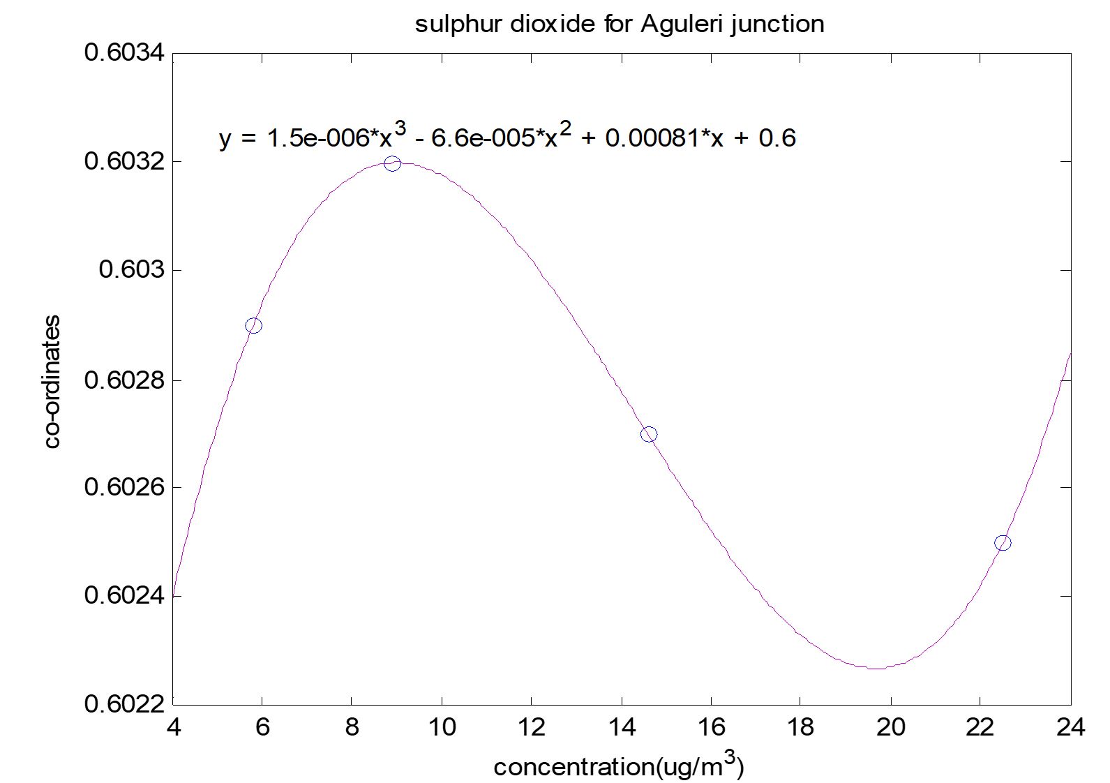
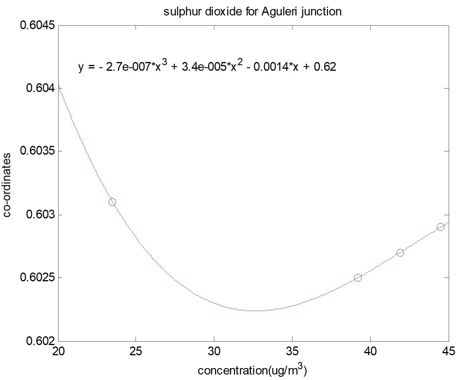
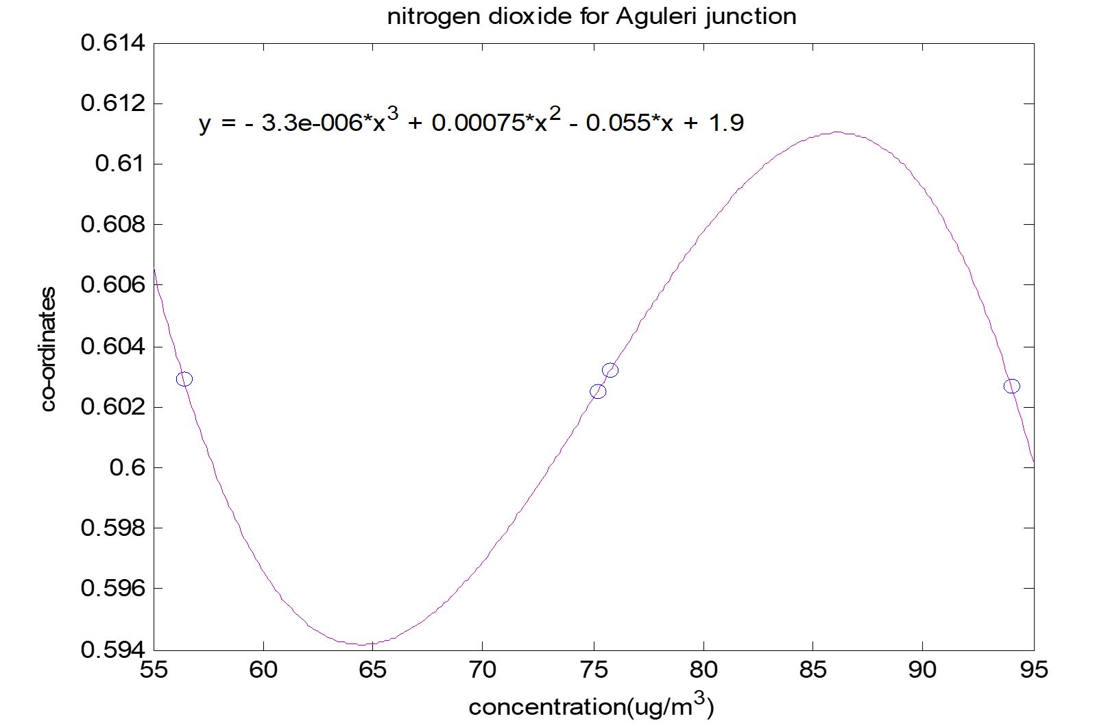
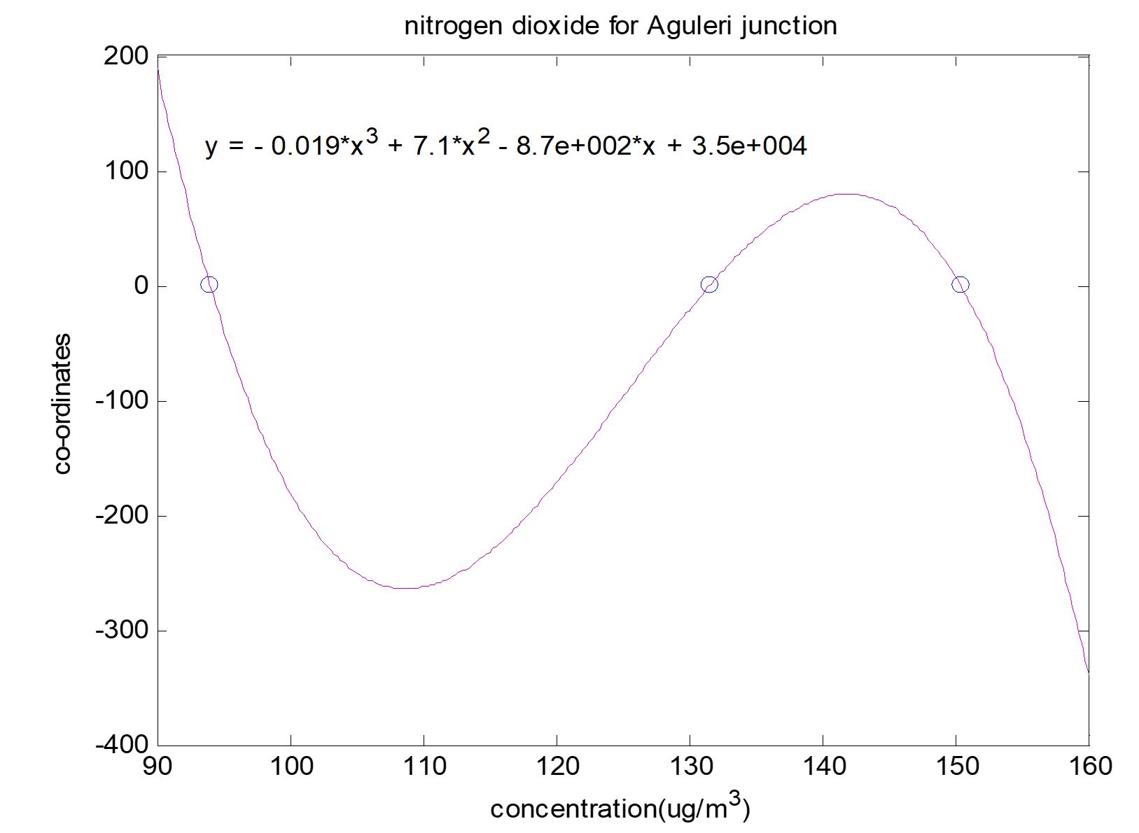
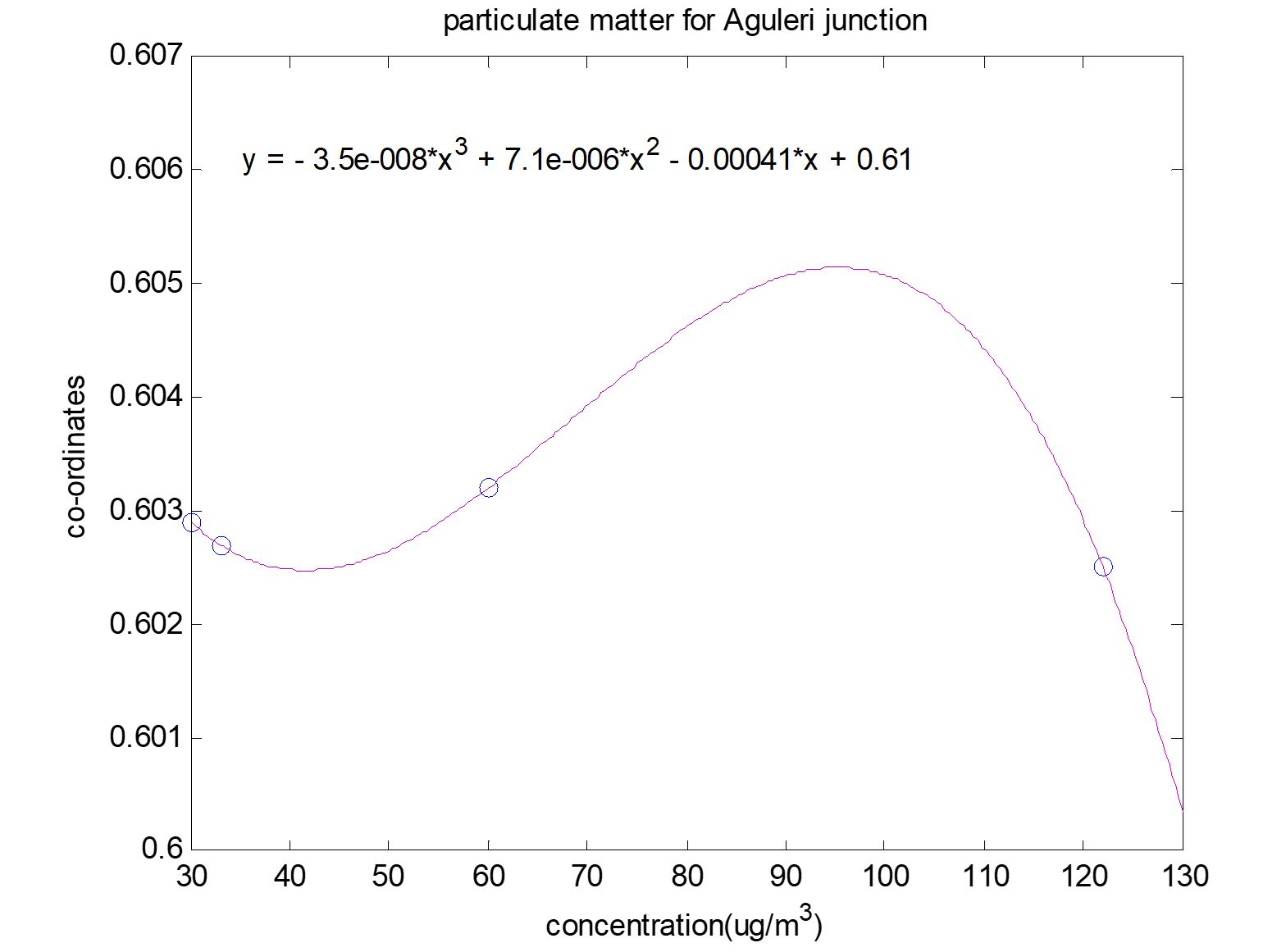
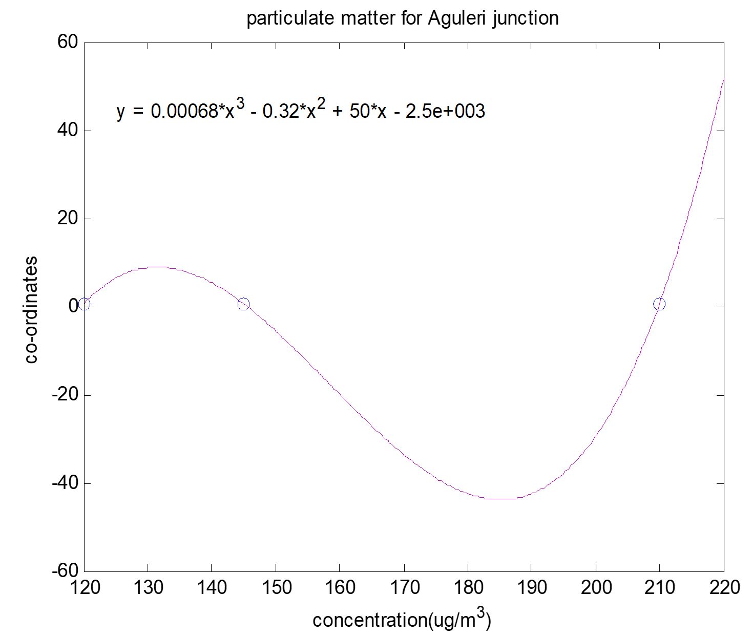
MATLAB-assisted fitted curves for variations in the concentration of SO2, NO2, and PM10 as a function of coordinates in the Aguleri study area during rainy and dry seasons are shown in Figure 2, Figure 3, Figure 4, Figure 5, Figure 6 and Figure 7 using the Aguleri Junction study location.
DISCUSSION
Evaluation of Pollution Models
The data generated revealed that the Ab Initio air pollution model developed from the fitted curves (Figure 2, Figure 3, Figure 4, Figure 5, Figure 6 and Figure 7) does not match constants from Ab Initio calculations closely enough in Table 6, Table 7, Table 8 and Table 9. This could be because Ab Initio calculations were an average of all variations at a station as a linear summation.
Constants from MATLAB fitted curves represent the effect of one parameter as a pollutant at a given time and across all locations of the study area.
Therefore, to a greater extent, the above plots represent a much more theoretical evaluation of pollution as a function of a single component and in tandem with the result of a non-point source event-based medium, which accounts for the simultaneous effects of all pollution indices.
Table 4
Summary of Pollutant Data in Aguleri during the Rainy Season
|
STATION |
SO2 (µg/m3) |
NO2 (µg/m3) |
PM10 (µg/m3) |
Relative Humidity % |
Wind Speed ms-1 |
Wind Direction (O) |
|
Aguleri Junction |
12.95 ± 0.01 |
75.20 ± 0.03 |
61.25 ± 0.01 |
73.50 ± 0.01 |
1.88 ± 0.01 |
233.20 ± 0.02 |
|
Ifite Aguleri |
7.85 ± 0.01 |
61.10 ± 0.01 |
32.00 ± 0.01 |
68.40 ± 0.01 |
1.47 ± 0.01 |
210.50 ± 0.02 |
|
Igboezuru Aguleri |
4.15 ± 0.02 |
47.00 ± 0.02 |
22.00 ± 0.02 |
66.90 ± 0.01 |
1.65 ± 0.02 |
236.90 ± 0.01 |
|
Okpu Aguleri |
3.00 ± 0.01 |
37.60 ± 0.01 |
20.00 ± 0.20 |
70.00 ± 0.02 |
1.50 ± 0.03 |
243.80 ± 0.01 |
|
Umuokpoto Aguleri |
2.90 ± 0.02 |
42.30 ± 0.20 |
28.00 ± 0.01 |
63.80 ± 0.01 |
1.16 ± 0.01 |
240.90 ± 0.02 |
|
Enugu Otu Aguleri |
0.97 ± 0.01 |
21.15 ± 0.01 |
10.25 ± 0.01 |
69.50 ± 0.02 |
1.25 ± 0.03 |
251.70 ± 0.02 |
|
Ezi Aguluotu Aguleri |
0.95 ± 0.02 |
11.75 ± 0.02 |
5.00 ± 0.01 |
74.10 ± 0.01 |
1.07 ± 0.01 |
193.80 ± 0.02 |
|
Umundeze Aguleri |
1.10 ± 0.02 |
14.10 ± 0.01 |
6.50 ± 0.01 |
68.30 ± 0.01 |
1.20 ± 0.02 |
175.50 ± 0.01 |
|
Amaeze Aguleri |
2.35 ± 0.01 |
44.65 ± 0.01 |
25.50 ± 0.01 |
68.50 ± 0.20 |
1.64 ± 0.01 |
197.30 ± 0.20 |
Table 5
Summary of Pollutant Data in Aguleri during the Dry Season
|
STATION |
SO2 (µg/m3) |
NO2 (µg/m3) |
PM10 (µg/m3) |
Relative Humidity % |
Wind Speed ms-1 |
Wind Direction (O) |
|
Aguleri Junction |
37.27 ± 0.01 |
131.60 ± 0.01 |
171.25 ± 0.01 |
62.90 ± 0.02 |
1.30 ± 0.01 |
202.75 ± 0.02 |
|
Ifite Aguleri |
18.30 ± 0.01 |
103.40 ± 0.01 |
104.50 ± 0.01 |
54.70 ± 0.01 |
1.79 ± 0.01 |
200.50 ± 0.02 |
|
Igboezuru Aguleri |
12.45 ± 0.02 |
63.45 ± 0.03 |
78.50 ± 0.02 |
53.50 ± 0.20 |
1.20 ± 0.01 |
224.75 ± 0.01 |
|
Okpu Aguleri |
10.45 ± 0.01 |
54.05 ± 0.01 |
59.50 ± 0.01 |
56.00 ± 0.02 |
1.31 ± 0.01 |
232.25 ± 0.01 |
|
Umuokpoto Aguleri |
11.15 ± 0.02 |
75.20 ± 0.03 |
69.75 ± 0.02 |
49.10 ± 0.01 |
0.76 ± 0.01 |
238.00 ± 0.02 |
|
Enugu Otu Aguleri |
6.82 ± 0.01 |
42.30 ± 0.01 |
30.00 ± 0.01 |
50.70 ± 0.01 |
0.64 ± 0.01 |
218.25 ± 0.03 |
|
Ezi Aguluotu Aguleri |
7.17 ± 0.02 |
47.00 ± 0.01 |
38.50 ± 0.01 |
52.60 ± 0.01 |
0.45 ± 0.01 |
168.50 ± 0.02 |
|
Umundeze Aguleri |
6.85 ± 0.01 |
63.45 ± 0.01 |
47.00 ± 0.01 |
54.60 ± 0.01 |
1.02 ± 0.01 |
136.00 ± 0.01 |
|
Amaeze Aguleri |
12.45 ± 0.01 |
98.70 ± 0.01 |
64.50 ± 0.01 |
52.70 ± 0.01 |
1.57 ± 0.01 |
124.00 ± 0.01 |
Table 6
Summary of Explicit Polynomials Obtained as Solutions (Aguleri, rainy season)
|
Station |
Pollution index model |
|
Aguleri junction |
0.6023–9.4×10⁻⁵SO2+1.6×10⁻⁵NO2+9.4×10⁻⁶PM10 |
|
Ifite Aguleri |
0.6039+3.5×10⁻⁵SO2+4.02×10⁻⁶NO2+9.6×10⁻⁶PM10 |
|
Igboezuru Aguleri |
0.6109+9.1×10⁻⁵SO2+3.0×10⁻⁶NO2–2.7×10⁻⁵PM10 |
|
Okpu Aguleri |
0.6575+2.52×10⁻³SO2–4.011×10⁻¹NO2+3.6×10⁻⁴PM10 |
|
Umuokpoto Aguleri |
0.6044–2.5×10⁻⁴SO2+1.9×10⁻⁵NO2+5.0×10⁻⁵PM10 |
|
Enugu Otu Aguleri |
0.7385–2.0×10⁻⁴SO2–5.6×10⁻⁴NO2+3.6×10⁻⁵PM10 |
|
Ezi Agulu Otu Aguleri |
0.6107–1.5×10⁻³SO2–8.5×10⁻⁵NO2+6.0×10⁻⁵PM10 |
|
Umundeze |
0.6049–5.0×10⁻⁴SO2–3.7×10⁻⁵NO2 |
|
Amaeze |
0.5944+1.2×10⁻⁴SO2–3.0×10⁻⁶NO2–3.3×10⁻⁵PM10 |
Table 7
Summary of Explicit Polynomials Obtained as Solutions (Aguleri, dry season)
|
Station |
Pollution index model |
|
Aguleri junction |
0.6020–1.5×10⁻⁵SO2+8.5×10⁻⁶NO2+1.2×10⁻⁶PM10 |
|
Ifite Aguleri |
0.4609+7.9×10⁻³SO2–6.1×10⁻⁶NO2+3.9×10⁻⁶PM10 |
|
Igboezuru Aguleri |
0.6092+4.0×10⁻⁶SO2+1.4×10⁻⁵NO2–9.0×10⁻⁵PM10 |
|
Okpu Aguleri |
0.6100–3.8×10⁻⁵SO2+6.0×10⁻⁶NO2–1.4×10⁻⁴PM10 |
|
Umuokpoto Aguleri |
0.6053+7.2×10⁻⁵SO2+2.0×10⁻⁶NO2–5.0×10⁻⁶PM10 |
|
Enugu Otu Aguleri |
0.7319+1.15×10⁻⁴SO2–2.5×10⁻⁵NO2–8.0×10⁻⁵PM10 |
|
Ezi Agulu Otu Aguleri |
0.6090+1.4×10⁻⁴SO2+2.4×10⁻⁵NO2–8.0×10⁻⁵PM10 |
|
Umundeze |
0.6054–7.4×10⁻⁴SO2–2.1×10⁻⁵NO2–5.0×10⁻⁵PM10 |
|
Amaeze |
0.5869–5.8×10⁻⁵SO2–5.3×10⁻⁶NO2+1.25×10⁻⁴PM10 |
Table 8
k Values obtained as simulated linearisation of pollution indices (Aguleri, rainy season)
|
Station |
K |
k1 |
k2 |
k3 |
|
Aguleri junction |
0.6023 |
–0.000094 |
0.000016 |
0.0000094 |
|
Ifite Aguleri |
0.6039 |
0.000035 |
0.00000402 |
0.0000096 |
|
Igboezuru Aguleri |
0.6109 |
0.000091 |
0.000003 |
–0.000027 |
|
Okpu |
0.6575 |
0.00252 |
–0.4011 |
0.00036 |
|
Umuokpoto Aguleri |
0.6044 |
–0.00025 |
0.000019 |
0.00005 |
|
Enugu Otu Aguleri |
0.7385 |
–0.0002 |
–0.00056 |
0.000036 |
|
Ezi Agulu Otu Aguleri |
0.6107 |
–0.0015 |
–0.000085 |
0.00006 |
|
Umundeze |
0.6049 |
–0.0005 |
–0.000037 |
0 |
|
Amaeze |
0.5944 |
0.00012 |
–0.000003 |
–0.000033 |
Table 9
k Values obtained as simulated linearisation of pollution indices (Aguleri, dry season)
|
Station |
K |
k1 |
k2 |
k3 |
|
Aguleri junction |
0.6020 |
–0.000015 |
0.0000085 |
0.0000012 |
|
Ifite Aguleri |
0.4609 |
0.0079 |
–0.0000061 |
0.0000039 |
|
Igboezuru Aguleri |
0.6092 |
0.000004 |
0.000014 |
0.000009 |
|
Okpu Aguleri |
0.6100 |
–0.000038 |
0.000006 |
–0.000014 |
|
Umuokpoto Aguleri |
0.6053 |
0.000072 |
0.000002 |
–0.000005 |
|
Enugu Otu Aguleri |
0.7319 |
0.000151 |
–0.000025 |
–0.00008 |
|
Ezi Agulu Out Aguleri |
0.6090 |
0.00014 |
0.000024 |
–0.00008 |
|
Umundeze Aguleri |
0.6054 |
–0.00074 |
–0.000021 |
–0.00005 |
|
Amaeze Aguleri |
0.5869 |
–0.000058 |
–0.0000053 |
0.000125 |
In order to achieve this, the pollution indices were treated as objects in geographical space and location and their respective positions were monitored by the application of GIS/GPS contour mapping of concentration densities, as shown below.
Application of GIS/GPS Mapping of Concentration Densities of Pollutants
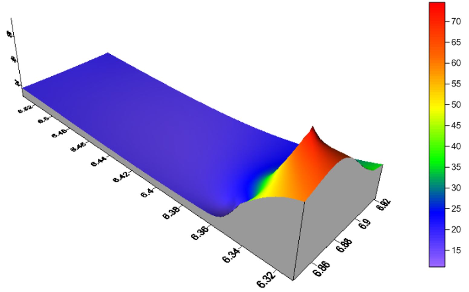
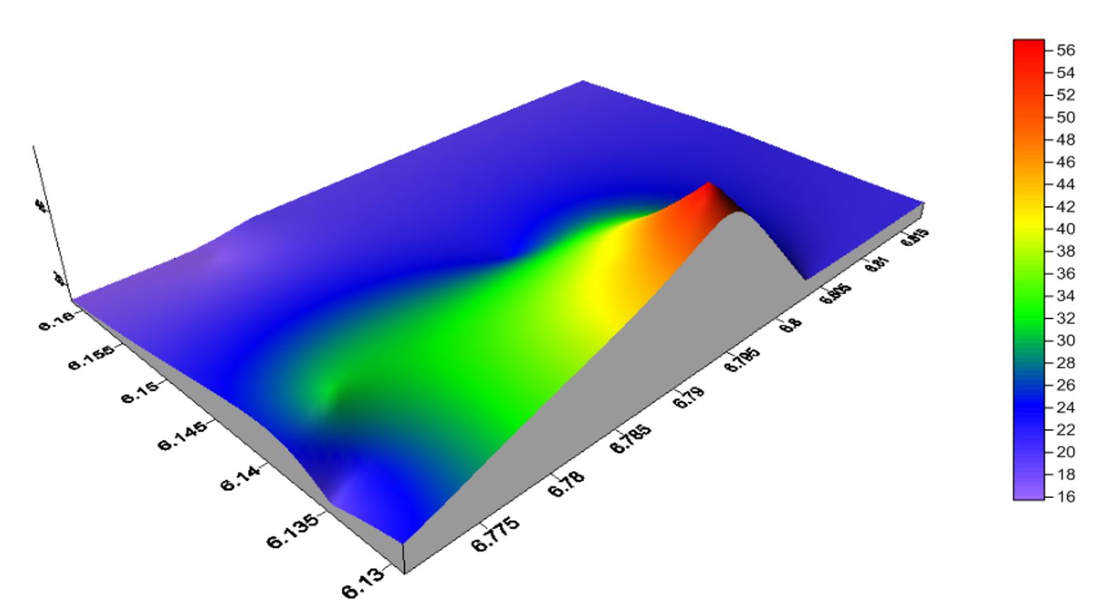
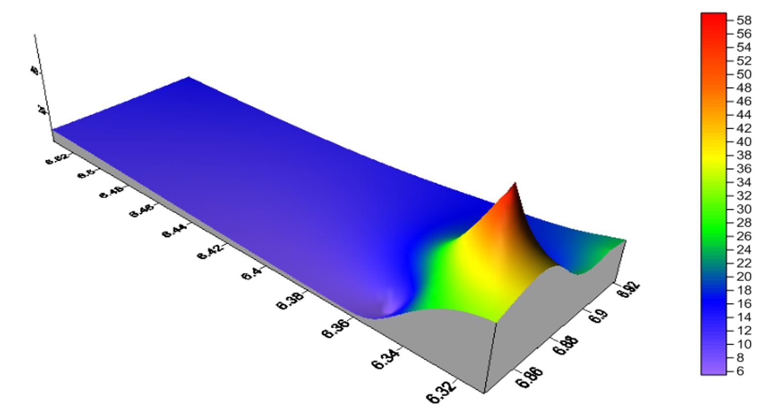
The concentration range of pollutants in Aguleri was 50%, as presented typically for Point 1 in Figure 8, Figure 9 and Figure 10. The corresponding three-dimensional (3D) surface plot in Figure 8 of the Aguleri junction was mononodal, and the area of very low NO2 concentration was clearly shown in the colour scheme. The surface plot in Figure 10 for PM10 at the same point in Aguleri was significant because the concentration of PM10 was shown to be very low at 6.43ºN and 6.92E.
The difference between the two GIS plots of NO2 was that the GIS plot of Figure 8 is two-dimensional, while the GIS surface plot of Figure 9 is 3D and gives a clearer view of the pollution vector density at the sampling stations for NO2 for Aguleri at point 1 for the rainy season. It gives the view of real life.
Effect of pollutant characteristics as a function of meteorological parameters
Air pollutant concentrations as a function of meteorological parameters, as shown in Figure 11 and Figure 12, revealed that over 50% of relative humidity affects the dispersion (concentrations) of the selected pollutants in all the nine sampling stations, and the variations were in the order of for the rainy season but for the dry season.
The wind speed was observed to be very low (< 10 m/s) and had little or no impact on the selected pollutants.
However, the effect of wind speed was more pronounced in the dry season than in the rainy season. Relative humidity varies directly with elevation; therefore, lower elevation gives lower relative humidity, less dispersion, and higher pollutant concentrations.
Many meteorological parameters vary inversely with air pollutant concentrations (Anyika et al., 2018; Rahman et al., 2006)
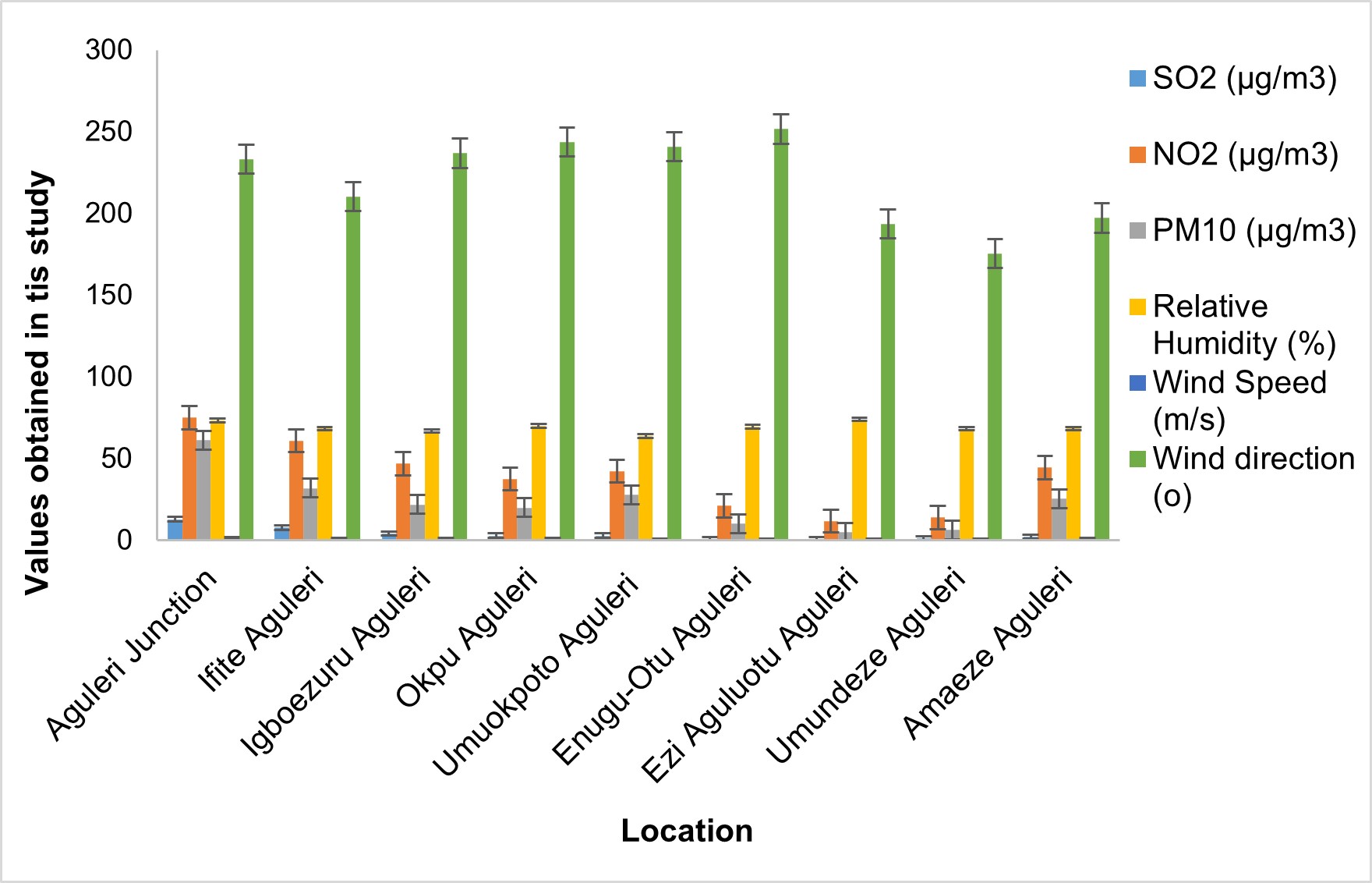
Figure 11 – Effect of meteorological parameters on the average concentration of pollutants during the rainy season
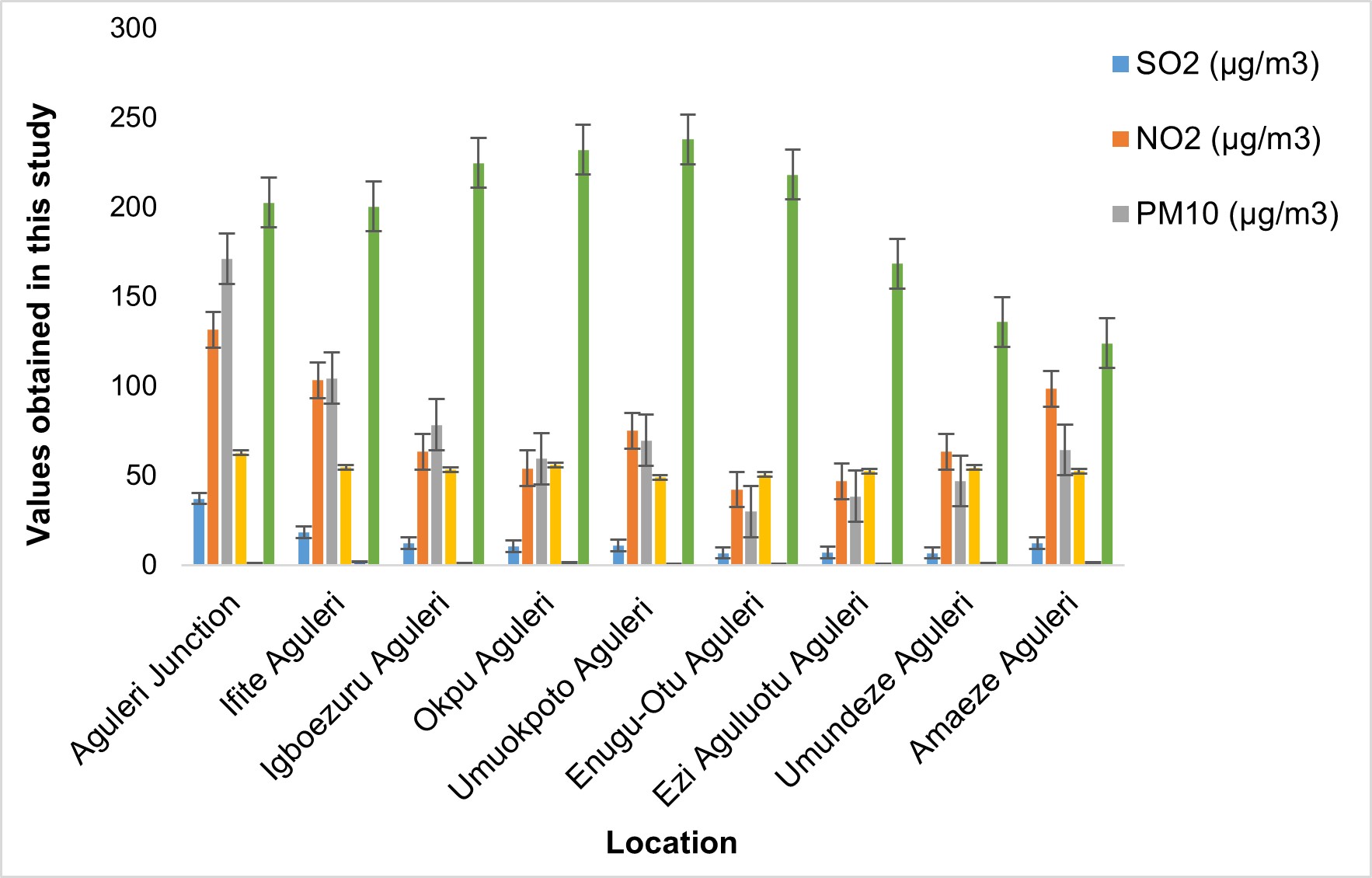
Figure 12 – Effect of meteorological parameters on the average concentration of pollutants during the dry season
AQI
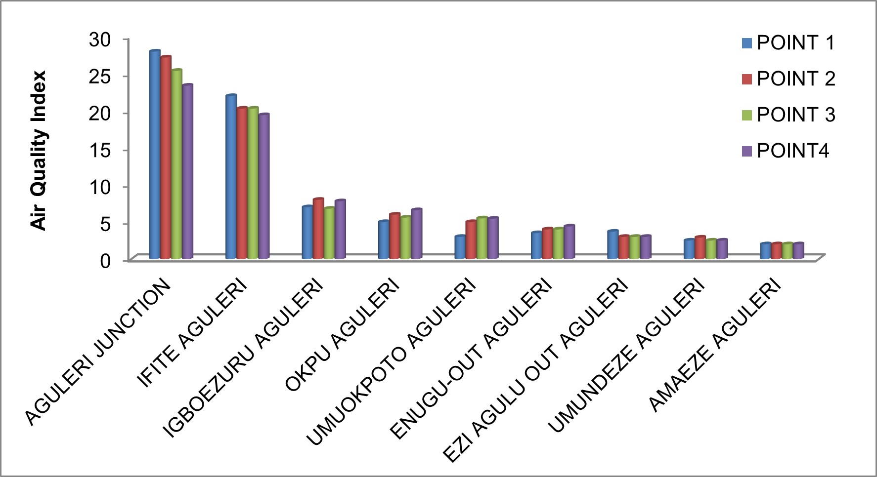
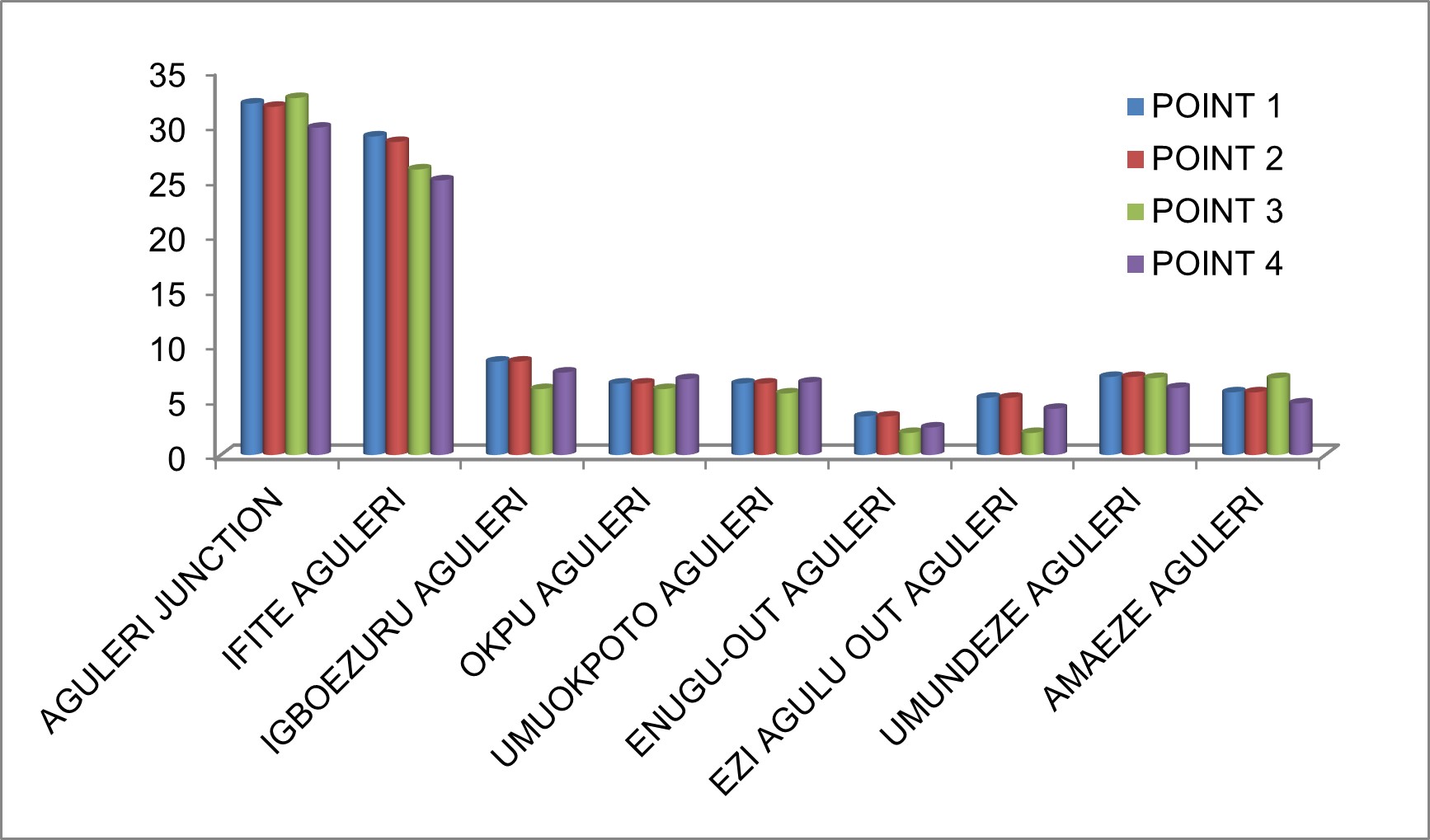
The results of the AQI, as presented in Table 10 and Table 11, Figure 13 and Figure 14, show that all the locations in both the rainy and dry seasons were below a 50 AQI rating.
A cursory look at the air quality of the study locations using the rating by USEPA (2000) for determining ambient air quality in Table 3 showed that the AQI rating for all the stations in the Aguleri study area for both rainy and dry seasons was very good (A category) with the exception of Aguleri Junction and Ifite Aguleri which had an AQI rating of good (B category).
The good AQI ratings of two areas suggest that these areas have fewer anthropogenic activities, while the very good AQI ratings of other areas suggest these areas have very few anthropogenic activities from very few vehicles and the absence of industries.
The AQI rating of good indicates no general health effect on the general public, but extreme measures must be taken to avoid incidences of hazardous activities.
Table 10
Air quality index of Aguleri (rainy season)
|
Sampling Stations |
Point 1 |
Point 2 |
Point 3 |
Point4 |
Description |
|
Aguleri Junction |
28.00 |
27.20 |
25.40 |
23.40 |
good |
|
Ifite Aguleri |
22.00 |
20.30 |
20.30 |
19.42 |
good |
|
Igboezuru Aguleri |
7.00 |
8.00 |
6.80 |
7.80 |
very good |
|
Okpu Aguleri |
5.00 |
6.00 |
5.60 |
6.60 |
very good |
|
Umuokpoto Aguleri |
3.00 |
5.00 |
5.50 |
5.45 |
very good |
|
Enugu-Out Aguleri |
3.50 |
4.00 |
4.00 |
4.40 |
very good |
|
Ezi Agulu Out Aguleri |
3.70 |
3.00 |
3.00 |
3.00 |
very good |
|
Umundeze Aguleri |
2.50 |
2.90 |
2.50 |
2.50 |
very good |
|
Amaeze Aguleri |
2.00 |
2.00 |
2.00 |
2.00 |
very good |
Table 11
Air quality index of Aguleri (dry season)
|
Sampling Stations |
Point 1 |
Point 2 |
Point 3 |
Point4 |
Description |
|
Aguleri Junction |
32.00 |
31.70 |
32.50 |
29.80 |
good |
|
Ifite Aguleri |
29.00 |
28.50 |
26.00 |
25.00 |
good |
|
Igboezuru Aguleri |
8.50 |
8.50 |
6.00 |
7.50 |
very good |
|
Okpu Aguleri |
6.50 |
6.50 |
6.00 |
6.90 |
very good |
|
Umuokpoto Aguleri |
6.50 |
6.50 |
5.60 |
6.60 |
very good |
|
Enugu-Out Aguleri |
3.50 |
3.50 |
2.00 |
2.50 |
very good |
|
Ezi Agulu Out Aguleri |
5.2 |
5.20 |
2.00 |
4.20 |
very good |
|
Umundeze Aguleri |
7.1 |
7.10 |
7.00 |
6.10 |
very good |
|
Amaeze Aguleri |
5.7 |
5.70 |
7.00 |
4.70 |
very good |
CONCLUSIONS
This study has shown that the evaluation of pollution models generated from ab initio constants obtained as an average of all variations at a station in a linear summation was more reliable than constants from fitted curves, which were a function of a single component. It has been shown that GIS contour surface plots used to obtain air pollution characteristics on surfaces gave more reliable data than tabulated values.
This study reveals that GIS vector density plots for air pollution characteristics can be used to predict air pollution as a function of industrial clustering. The solution of model polynomials representing air pollution characteristics can be used to predict pollution attributes as a function of data space. The predictor constants generated by solving the model simultaneous equations using MATLAB 7.9 representing modifiers of air pollution were efficient. The study has demonstrated the predictive power of GIS/GPS in the rendering of air pollution in terms of objects in data space and their interaction with meteorological parameters. The meteorological variables like relative humidity serve as effective scavengers for SO2, NO2 and PM10 pollutants and vary in both rainy and dry seasons. The information obtained from this study could lead to best environmental management practices and the establishment of efficient pollution control departments, as in many developed and advanced countries. However, some limitations encountered in this study were predominantly difficulties in the collection of the samples due to the hostility of youth in Aguleri and difficulties measuring with instruments and digital sensors from the various environmental agencies. In future air pollution assessments, this study recommends using more mathematical analysis involving polynomial equations as formulated, which should be performed by iteration.
Author Contributions: Conceptualization by ALC and OC; methodology by ALC; analysis by ALC; investigation by ALC; resources ALC; data curation by ALC and OC; writing by ALC and OC, review by OC. All authors declare that they have read and approved the publication of the manuscript in this present form.
Funding: There was no external funding for this study.
Acknowledgments: The authors deeply appreciate the assistance of the Department of Mechanical Engineering, Federal University of Technology Owerri for providing apparatuses used for this sophisticated study and the staff and management Imo State Environmental Protection Agency (ISEPA) for providing gas monitors.
Conflicts of Interest: The authors declare non-existence of any interest(s).
REFERENCES
Abam, F.I.; Unachukwu, G.O. Vehicular Emissions and Air Quality Standards in Nigeria. European Journal of Scientific Research. 2009, 34, 550-560.
Abdul-Lateef, B.; Abdulwaheed, T.; Lavania, B.; Naheem, A. A review of the inter-correlation of climate change, air pollution and urban sustainability using novel machine learning algorithms and spatial information science. Urban Climate. 2021, 40, 100989. https://doi.org/10.1016/j.uclim.2021.100989
Abdulraheem, K.A.; Adeniran, J.A.; Aremu, A.S.; Yusuf, M.N.O.; Yusuf, R.O.; Odediran, E.T.; Sonibare, J.A.; Du, M. Quantifications and predictions of sectoral pollutants emissions in Nigeria from 1980 to 2050. Environmental Monitoring and Assessment. 2023, 195, 398. https://doi.org/10.1007/s10661-022-10872-5.
Abulude, F.O.; Oyetunde, J.G.; Feyisetan, A.O. Air Pollution in Nigeria: A Review of Causes, Effects, and Mitigation Strategies. Continental Journal of Applied Sciences. 2024, 19, 1-23. https://doi.org/10.5281/zenodo.10633771
Anyika, L.C.; Alisa, C.O.; Nkwoada, A.U.; Opara, A.I.; Ejike, E.N.; Onuoha, G.N. GIS and MATLAB modeling of criteria pollutants: a study of lower Onitsha basin during rains. Journal of Science, Technology and Environmental Informatics. 2018, 06, 443-457. https://doi.org/10.18801/jstei.060118.47
Augustine, C. Impact of Air Pollution on the Environment in Port Harcourt, Nigeria. Journal of Environmental Science and Water Resources. 2012,1, 46-51.
Badach, J.; Voordeckers, D.; Nyka, L.; Acker, M.V. A framework for Air Quality Management Zones-Useful GIS-based tool for urban planning: Case studies in Antwerp and Gdańsk. Building and Environment. 2020, 106743. https://doi.org/10.1016/j.buildenv.2020.106743
Balogun, I.A.; Adeyewa, D.Z.; Balogun, A.A.; Morakinyo, T.E. Analysis of Urban expansion and Land use changes in Akure, Nigeria, using remote sensing and geographic information system (GIS) techniques. Journal of Geography and Regional Planning. 2011, 4, 533-541.
Borah, J.; Mohd, S.; Mohd, N.; Cayetano, M.G.; Majumdar, S.; Ghayvat, H.; Srivastava, G. Hybrid-Ensemble Internet-of-Things sensing unit model for air pollution control. Institute of Electrical and Electronics Engineers Sensors Journal. 2024, 21558-21565. https://doi.org/10.1109/JSEN.2024.3397735
Chaminé, H.I.; Pereira, A.J.S.C.; Teodoro, A.C.; Teixeira, J. Remote sensing and GIS applications in earth and environmental systems sciences. SN Applied Sciences. 2021, 3, 870. https://doi.org/10.1007/s42452-021-04855-3
Chengyue, Z.; Kannan, M.; Kechun, L.; Yun, Z. Role of atmospheric particulate matter exposure in COVID-19 and other health risks in human: A review. Environmental Research. 2021, 198, 111281. https://doi.org/10.1016/j.envres.2021.111281
Daful, M.G.; Adewuyi, T.O.; Muhammad, M.N.; Oluwole, O.A.; Dadan-Garba, A.; Ezeamaka, C.K. Assessment of the spatial relationship between air pollutants in Kaduna metropolis. Nigeria. Journal of Sustainable Development. 2020, 13, 204. https://doi.org/10.5539/jsd.v13n4p204
Dimari, G.A.; Hati, S.S.; Waziri, M.; Maitera, O.N. Pollution Synergy from Particulate Matter sources: The Harmattan, Fugitive Dust and Combustion Emissions in Maiduguri Metropolis, Nigeria. European Journal of Scientific Research. 2008, 23, 465-473. http://dx.doi.org/10.13140/2.1.3407.6160
Egbuna, C.; Amadi, C.N.; Patrick-Iwuanyanwu, K.C.; Ezzat, S.M.; Awuchi, C.G.; Ugonwa, P.O.; Orisakwe, O.E. Emerging pollutants in Nigeria: A systematic review. Environmental Toxicology and Pharmacology. 2021, 85. https://doi.org/10.1016/j.etap.2021.103638
Ediagbonya, T.F.; Tobin, A.E. Air Pollution and Respiratory Morbidity in an urban Area of Nigeria. Greener Journal of Environment Management and Public Safety. 2013, 2, 010-015.
Firouraghi, N.; Kiani, B.; Jafari, H.T.; Learnihan, V.; Salinas-Perez, J.A.; et al. The role of geographic information system and global positioning system in dementia care and research: a scoping review. International Journal of Health Geographics. 2022, 21, 8. https://doi.org/10.1186/s12942-022-00308-1
Gerard, H. Carbon monoxide’s potential comeback as a key air pollutant. The Lancet Planetary Health. 2021, 5, e177-e178. https://doi.org/10.1016/s2542-5196(21)00052-8
Google earth. Retrieved January 15, 2018, from Google earth: https://www.google.com/earth/
Ilmas, B.; Mir, K.A.; Khalid, S. Greenhouse gas emissions from the waste sector: a case study of Rawalpindi in Pakistan. Carbon Management. 2018, 9, 645-654. https://doi.org/10.1080/17583004.2018.1530025
Jiayu, L.; Haoran, L.; Yehan, M.; Yang, W.; Ahmed, A.; Chenyang, L.; Pratim, B. Spatiotemporal distribution of indoor particulate matter concentration with a low-cost sensor network. Building and Environment. 2018, 127, 138-147. https://doi.org/10.1016/j.buildenv.2017.11.001
Jyethi, D.S. Air Quality: Global and Regional Emissions of Particulate Matter, SOx, and NOx. In Plant Responses to Air Pollution, Kul Shrestha, U., Saxena, P. (eds). Springer, Singapore, 2016, 5-19. https://doi.org/10.1007/978-981-10-1201-3_2
Khan, Z.R.; Jehangir, A. Geostatistical Methods and Framework for Pollution Modelling. In Geospatial Analytics for Environmental Pollution Modeling, Mushtaq, F., Farooq, M., Mukherjee, A. B., Ghosh Nee Lala, M. (eds), Springer, Cham, 2023, 33-56. https://doi.org/10.1007/978-3-031-45300-7_2
Khaslan, Z.; Nadzir, M.S.M.; Johar, H.; Siqi, Z.; Sulong, N.A.; Mohamed, F.; Majumdar, S.; Suris, F.N.A.; Hawari, N.S.S.L.; Borah, J. Utilizing a low-cost air quality sensor: Assessing air pollutant concentrations and risks using low-cost sensors in Selangor, Malaysia. Water, Air and Soil Pollution. 2024, 235, 229. https://doi.org/10.1007/s11270-024-07012-9
Knepnick, I.A.; Sebastian, L. Environmental Working paper 31, Washington D.C. World Bank, 1990.
Lokeshwari, N.; Sriniketham, G.; Hegde, V.S. Air Quality Management – A Review. Middle East Journal of Scientific Research. 2014, 21, 1061-1070. https://doi.org/10.5829/idosi.mejsr.2014.21.07.21225
Luo, M.; Liu, X.; Legesse, N.; Liu, Y.; Wu, S.; Han, F.X.; Ma, Y. Evaluation of Agricultural Non-Point Source Pollution: A Review. Water, Air, and Soil Pollution. 2023, 234, 657. https://doi.org/10.1007/s11270-023-06686-x
Manisalidis, I.; Stavropoulou, E.; Stavropoulos, A.; Bezirtzoglou, E. Environmental and Health Impacts of Air Pollution: A Review. Frontier in Public Health. 2020, 8, 14. https://doi.org/10.3389/fpubh.2020.00014
Matejicek, L. Spatial modelling of air pollution in urban areas with GIS: a case study on integrated database development. Advances in Geosciences. 2005, 4, 63-68.
Mahmud, K.; Mitra, B.; Uddin, M.S.; Hridoy, Al-E. E.; Aina, Y.A.; Abubakar, I.R.; Rahman, S.M.; Tan, M.L.; Rahman, M.M. Temporal assessment of air quality in major cities in Nigeria using satellite data. Atmospheric Environment: X. 2023, 20, 100227. https://doi.org/10.1016/j.aeaoa.2023.100227
Najibullah, H.Z. GIS, remote sensing and GPS: Their activity, integration and fieldwork. International Journal of Applied Research. 2020, 6, 328-332.
Obisesan, A.; Weli, V.E. Assessment of air quality characteristics across various land-uses in Port Harcourt metropolis. Journal of Environmental Management. 2019, 2, 106.
Omofonmwan, S.I.; Osa-Edoh, G.L. The Challenges of Environment Problems in Nigeria. Journal of Humidity and Ecology. 2008, 23, 53-57.
Omokpariola, D.O.; Nduka, J.N.; Omokpariola, P.L. Short-term trends of air quality and pollutant concentrations in Nigeria from 2018–2022 using tropospheric sentinel-5P and 3A/B satellite data. Discover Applied Science. 2024, 6, 182. https://doi.org/10.1007/s42452-024-05856-8
Palomera, J.; Alvarez, B.; Echeverria, S.; Hernandez, E.; Alvarez, P.; Villegas, R. Photochemical assessment monitoring stations program adapted for ozone precursors monitoring network in Mexico City. Atmosphere. 2016, 29, 169-188. https://doi.org/10.20937/ATM.2016.29.02.06
Park, D.; Kwon, S.B.; Cho, Y. Development and Calibration of a Particulate Matter Measurement Device with a Wireless Sensor Network function. International Journal of Environmental Monitoring and Analysis. 2013, 1, 15-20.
Patra, A.K.; Gautam, S.; Majumdar, S.; et al. Prediction of particulate matter concentration in an opencast copper mine in India using artificial neutral model. Air Quality Atmospheric Health. 2016, 9, 697-711. https://doi.org/10.1007/s11869-015-0369-9
Pilla, F.; Broderick, B. A GIS model for personal exposure to PM10 for Dublin commuters. Sustainable Cities and Society. 2015, 15, 1-10. https://doi.org/10.1016/j.scs.2014.10.005
Rahman, M.; Kabir, F.; Begum, B.A.; Biswas, S.K. Monitoring and Trend Analysis of Air-Borne Particulate Matter (PM10 and PM2.5) at Major Host-Spot Areas: Mohakhali and Farm gate in Dhaka City. Journal of Chemical Engineering. 2006, 24, 61-67.
Raju, P.; Partheeban, P.; Hemamalini, R. Urban mobile air quality monitoring using GIS, GPS, sensors and internet. International Journal of Environmental Science and Development. 2012, 3, 324-327. https://doi.org/10.7763/IJESD.2012.V3.240
Robert, O.P.; Rahman, M.; Honda, K.; Strestha, A.; Vaseashta, A. SnO2 gas sensors and geo-informatics for air pollution monitoring. Journal of Optoelectronics and Advanced Materials. 2011, 13, 560-564.
Seham, S.; Al-Alola, I.I.; Alkadi, H.M.; Alogayell, S.A.; Mohamed, I.Y.I. Air quality estimation using remote sensing and GIS-spatial technologies along Al-Shamal train pathway, Al-Qurayyat City in Saudi Arabia. Environmental and Sustainability Indicators. 2022, 15, 100184. https://doi.org/10.1016/j.indic.2022.100184
Tawari, C.C.; Abowei, J.F.N. Air Pollution in the Niger Delta Area of Nigeria. International Journal of Fisheries and Aquatic Sciences. 2012, 1, 94-117.
Tella, A.; Balogun, A.L. GIS-based air quality modelling: spatial prediction of PM10 for Selangor State, Malaysia using machine learning algorithms. Environmental Science and Pollution Research. 2022, 29, 86109-86125. https://doi.org/10.1007/s11356-021-16150-0
Thakur, J.K.; Singh, S.K.; Ekanthalu, V.S. Integrating remote sensing, geographic information systems and global positioning system techniques with hydrological modeling. Applied Water Science. 2017, 1595-1608. https://doi.org/10.1007/s13201-016-0384-5
Utbah, R.; Mohd, S.; Mohd, N.; Siti, Z.; Abdullah, S.; Sharifah, B.; Izzati, W.; et al. Evaluations of Low-cost Air Quality Sensors for Particulate Matter (PM2.5) under Indoor and Outdoor Conditions. Sensors and Materials. 2023, 35, 2881-2895.
Verma, S.; Gangwar, T.; Singh, J.; Prakash, D.; Payra, S. Urban Air Quality Monitoring and Modelling Using Ground Monitoring, Remote Sensing, and GIS. In Geospatial Analytics for Environmental Pollution Modeling, Mushtaq, F., Farooq, M., Mukherjee, A.B., Ghosh Nee Lala, M. (eds), Springer, Cham, 2023, 213–247. https://doi.org/10.1007/978-3-031-45300-7_9
USEPA. United State Environmental Protection Agency. Air Quality Index for Priority Pollutants. United states Environmental Protection Agency, Washington DC., USA, 2000.
WHO. World Health Organization. Ambient (Outdoor) Air Quality and Health. 2022. https://www.who.int/news-room/fact-sheets/detail/ambient-(outdoor)-air-quality-and-health
Yalwaji, B.; John-Nwagwu, H.O.; Sogbanmu, T.O. Plastic pollution in the environment in Nigeria: A rapid systematic review of the sources, distribution, research gaps and policy needs. Scientific African. 2022, 16, e01220. https://doi.org/10.1016/j.sciaf.2022.e01220
Yerramilli, A.; Rao Dodla, V.B.; Yerramilli, S. Air Pollution, Modeling and GIS based Decision Support Systems for Air Quality Risk Assessment, In Advanced air pollution, Farhad Nejadkoorki, Iran. IntechOpen. 2011. http://dx.doi.org/10.5772/22055
Yorkor, B.; Leton, T.; Ugbebor, J. Prediction and modeling of seasonal concentrations of air pollutants in semi-urban region employing artificial neural network ensembles. International Journal of Environment and Pollution Research. 2017, 5, 1-18.
Yoo, M.P. A GPS-enabled portable air pollution sensor and web-mapping technologies for field-based learning in health geography. Journal of Geography in Higher Education. 2022, 46, 241-261. https://doi.org/10.1080/03098265.2021.1900083
Zezhi, P.; Bin, Z.; Diwei, W.; Xinyi, N.; Jian, S.; Hongmei, X.; Junji, C.; Zhenxing, S. Application of machine learning in atmospheric pollution research: A state-of-art review. Science of The Total Environment. 2024, 910, 168588. https://doi.org/10.1016/j.scitotenv.2023.168588
Zhu, K.; Chen, Y.; Zhang, S.; Yang, Z.; Huang, L.; Lei, B.; Li, L.; Zhou, Z.; Xiong, H.; Li, X. Identification and prevention of agricultural non-point source pollution risk based on the minimum cumulative resistance model. Global Ecology and Conservation. 2020, 23, e01149. https://doi.org/10.1016/j.gecco.2020.e01149
Academic Editor: Dr. Iuliana MOTRESCU
Publisher Note: Regarding jurisdictional assertions in published maps and institutional affiliations ALSE maintain neutrality.

